How I made acetate
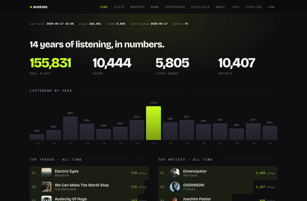
An acetate is the one-off reference disc a mastering engineer cuts before an album goes to press, a private pressing of the real thing. This is mine: a personal archive of 155,831 plays across 14 years of Spotify, with its own stats engine, its own playlist robots, an agent you can interrogate, and a 3D map of every song I've ever loved, embedded by a neural network that listens to each one.
It runs on a small box in my house. Spotify can't delete it, redesign it, or decide the feature I use isn't worth maintaining. Here's how it works, at whatever level of nerd you're comfortable with.
Why build this at all
Two reasons. First: my Liked Songs became a 5,676-track dumping ground , a write-only pile that no amount of discipline was going to curate. What I actually wanted was boring automation: playlists that build themselves from how I actually listen, monthly archives, genre shelves, "you loved this in 2016 and forgot it exists."
Second: in late 2024 Spotify turned off the APIs that made this hobby possible for new apps. Audio features (energy/danceability/valence): 403. Recommendations: 403. Related artists: 403. Artist genres: silently emptied. Even reading your own Discover Weekly returns a 404 now, as if it doesn't exist. I would have to compute the analysis myself from things they can't take away: my own listening history, open data, and the audio itself.
The data spine
Everything sits on one SQLite file. The thesis: at personal scale
(hundreds of thousands of rows, one user) a single WAL-mode SQLite file outruns any client-server
database you'd deploy, backs up with cp, and will still open in thirty years.
Around it, the architecture is just "things that write in" and "things that read out":
Sources
Spotify APIrecently-played poll · 15 min GDPR exportevery play since 2012 Deezer30s preview audio Last.fmtags · co-listening MusicBrainzrecording MBIDsone sqlite file
play_eventsthe listening log *_snapshotsappend-only backups recording_statscanonical per-song rollup embeddingsfloat32 blobs, 1280-d recording_stylesdiscogs400 top-8Consumers
dashboardstats · wrapped · gems playlist robotsmonthly · gems · smart chat agentSQL + similarity tools Hyperspacethe 3D mapThe full history came from the GDPR "extended streaming history" export, every play since 2012 with timestamps and how many milliseconds I actually listened. A poller tops it up every 15 minutes from the recently-played endpoint (one of the survivors), deduping against the export watermark, so history accumulates forever with no gaps.
Backups are append-only snapshots: playlists and liked songs are content-hashed each run and a full snapshot is written only when the hash changes. That gives a deletion trace, when a playlist disappears or a song un-likes itself (it happens), the record of what-was survives.
The subtle one is canonicalization. Spotify hands out a different track ID for the same recording on the single, the album, and the compilation, and your plays scatter across them. A normalization pass collapses ~48k raw track IDs into 43,077 logical recordings, and every stat joins through that map, otherwise a favorite's play count splits across three IDs and it quietly falls out of every top list.
The genre saga, or: how metadata broke my heart
The original north star was simple: genre playlists that maintain themselves. A "melodic techno" shelf that quietly accumulates my favorites without me curating anything. I assumed, foolishly, that knowing what genre a song is was the solved part, and the playlist plumbing would be the work. It went in four acts.
Act one: ask Spotify. Tracks have no genre field at all, fine, artists do. Except
by the time I got here, the artist genres[] array had been quietly emptied for new
API apps. The field still exists; it just returns nothing. A genre system where nothing has a
genre.
Act two: ask the crowd. Last.fm tags, cached with their weights and cleaned through a denylist (no, "seen live" is not a genre; neither is "belgian"). And this genuinely works, for genres the crowd agrees on. Deep house, trance, dubstep, downtempo: clean, dense, accurate. Then I validated it against my own hand-built melodic-techno playlist and got the number that reframed the whole project: only 9% of those tracks carry the literal tag "melodic techno". Crowd tags are sparse exactly where taste is specific. The genres you care enough to name are the ones nobody agrees on.
Act three: ask a language model. The plan on the bench: batch-classify tracks from artist + title + whatever tags exist, with my own authored playlists as ground truth and eval set. Cost napkin said a few dollars for the whole library on a small model. Plausible! Still plausible, it may yet run as the final arbiter. But it felt like asking someone to guess the genre from the album cover: the one thing every approach so far had in common was that none of them had heard the song.
Act four: the reframe. Genre isn't metadata. It's a property of the audio. If nothing in the metadata economy would tell me what my music sounds like, the move was to compute it from the sound itself, which is where this stopped being a data-cleaning project and became the fun part.
Teaching it to hear
If the tags won't describe the music, the audio will. Every track in the analysis universe (liked, or played ≥5 times, 8,689 recordings) goes through a pipeline that ends with the machine having listened to my entire library:
The audio comes from Deezer's public preview API, looked up by ISRC, the industry's serial number for a recording, which Spotify still hands out. Exact match, no fuzzy search, no account, about 10% misses. And here's the part that sounds wrong but isn't: a 128 kbps 30-second clip is lossless to the model. The embedding network resamples everything to 16 kHz mono before it listens, every argument about audio quality dies at the resampler. The same clips double as click-to-play previews in the map.
The model is discogs-effnet from MTG, the Music Technology Group at Universitat Pompeu Fabra in Barcelona, the lab behind the Essentia audio-analysis stack and much of the last two decades of music-information-retrieval research, an EfficientNet trained against Discogs metadata. One forward pass gives both a 1280-dimensional "what this sounds like" vector and scores over 400 Discogs styles, a taxonomy deep enough to know Tech House from Deep House from Progressive House, i.e. the distinctions Last.fm shrugs at. It nails my library: the Kygo remix comes back "Tropical House", Emancipator comes back "Downtempo", and on a 30-second clip it takes 0.8 seconds per track on a laptop.
Under the hood: discogs-effnet
Worth opening this one up, because every model in this project follows the same recipe with different choices at each step.
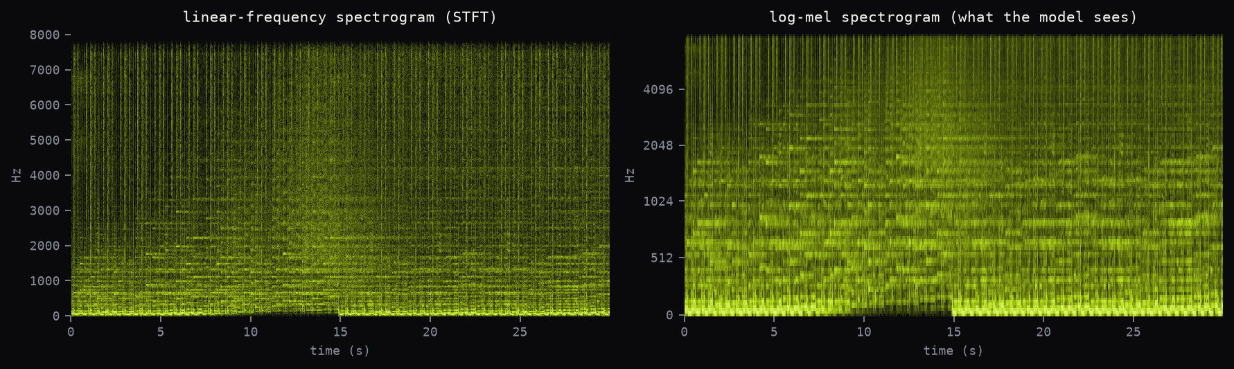
Step one: sound becomes a picture. The network never sees a waveform. The audio is converted to a log-mel spectrogram, time on the x-axis, frequency on the y-axis, brightness = energy, with the frequency axis warped onto the mel scale, which spaces frequencies the way human hearing does (we can tell 100 Hz from 200 Hz easily; 7,100 from 7,200 not at all):
The log on the energy axis does the same trick for loudness. Two perceptual warps and sound is now an image whose textures are musical texture, kick drums are bright columns, pads are horizontal washes, hi-hats are high-frequency stubble. Here it is for real, on the specimen this whole section dissects: Corren Cavini's “Listen to the Silence”, a deep cut by design: modest streaming numbers, a few hundred Last.fm listeners, and no crowd consensus on what to call it. Tracks like that are the reason this pipeline exists, the hits already have all the metadata they'll ever need.
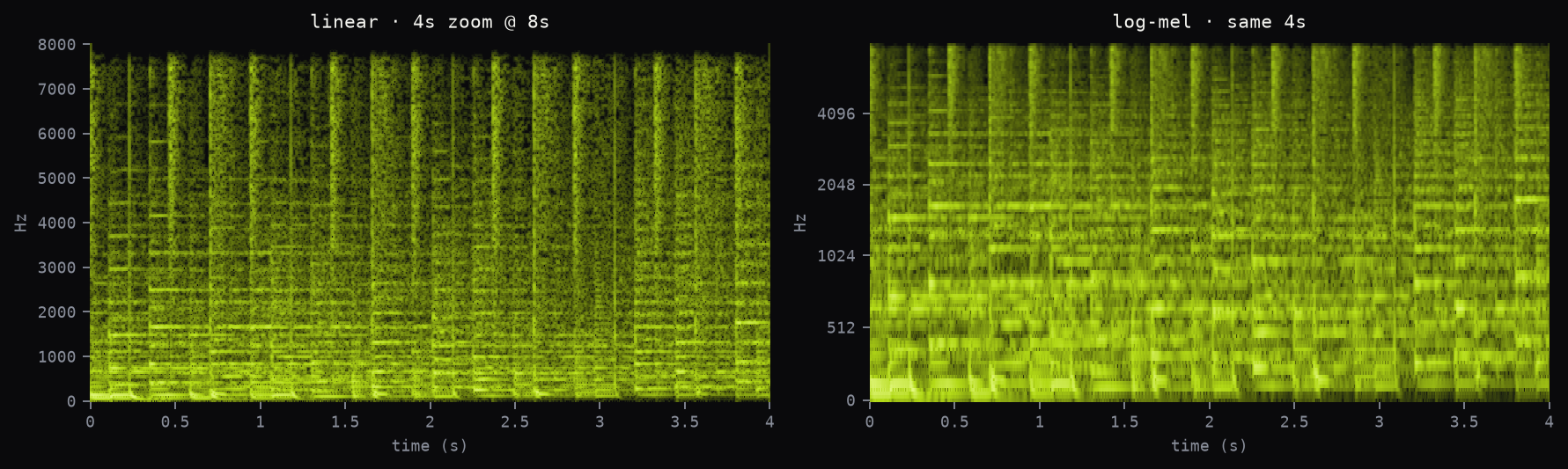
Zoom in four seconds and the two representations really argue their case, the linear panel spends its pixels on empty treble; in the log-mel panel nearly the whole canvas carries usable texture. Same audio, same information budget, spent where ears actually listen:
Step two: an image classifier looks at it. The backbone is EfficientNet-B0, a 2019 Google image-classification network and the smallest member of a family built around one idea, compound scaling: instead of growing depth, width, or input resolution independently, all three scale together by a fixed rule, and B0 is the base case the rule starts from. It's tiny by modern standards, about five million parameters, arranged as a stem convolution plus 16 MBConv blocks in seven stages. An MBConv block is the inverted-residual bottleneck from MobileNetV2: a cheap depthwise convolution filters each channel separately while 1×1 convolutions do the mixing, which deletes most of the FLOPs of an ordinary convolution. Each block also carries a squeeze-and-excitation module , a small gate that averages every channel down to one number and learns which channels to amplify. Attention, at 2019 prices. The "efficient" is real: it's why a laptop CPU does this at 0.8s/track.
The network convolves over spectrogram tiles exactly as it would over photos of dogs , edges, textures, motifs, except here an "edge" is a kick transient and a "texture" is a pad. After the last stage, global average pooling collapses whatever spatial grid remains into one vector of 1,280 numbers: the penultimate layer, and the embedding we keep. Everything past it, the classifier head, gets read once for the style scores and otherwise ignored; the representation, not the verdict, is the product.
Step three: the supervision decides what the space means. This network was trained by MTG on ~3.3 million tracks matched to Discogs release metadata, learning to predict the release's styles. That objective is the whole personality of the model: to get good at distinguishing Deep House from Tech House from Progressive House, the 1280-d layer is forced to organize itself around genre-relevant texture. The embedding space is genre-shaped because genre was the exam. (Contrast: self-supervised models like MERT never see a genre label and organize around acoustic structure instead, different exam, different space; that comparison is a future entry in this notebook.) The discogs400 head on top is just a small classifier reading the embedding, which is why one forward pass yields both the vector and the 400 style scores nearly for free.
Step four: patches, then pooling. The network doesn't hear a whole clip at once. It slides over the spectrogram in ~3-second patches, embeds each one, and the track's vector is the mean over its N patches:
Mean-pooling throws away the song's structure, the drop and the intro average into one point, which is exactly right for "what does this track sound like overall" and exactly wrong for anything about arrangement. And you can see exactly what's being thrown away. Here's the same track in full, not the 30-second excerpt:
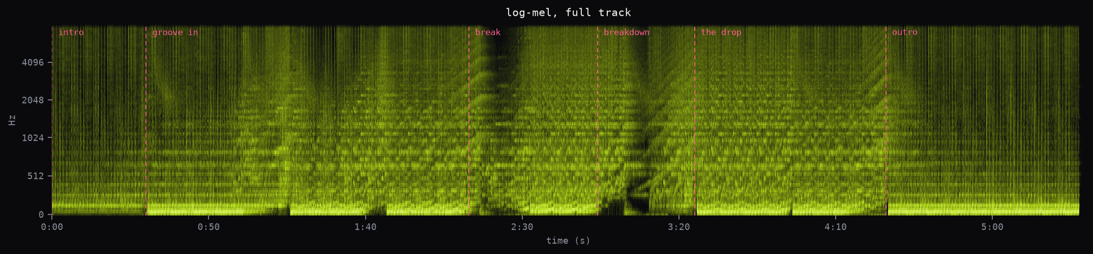
That arc, tension built over minutes and spent in one bar, is the entire craft of the genre, and it is invisible at every level of this pipeline: absent from the 30-second preview, absent from the model's ~3-second patches, and averaged into mush by the pooling. For "overall track vibe", genre, playlisting, the map, that's fine, even correct. But structure is its own signal (a DJ tool and a radio edit of the same song are different objects), and the fix is already latent in the pipeline: the patches exist, they're just being averaged. A per-section index, intro vectors, drop vectors, "find me tracks whose breakdown sounds like this", is the natural sequel, and it pairs with the text space from the next section: CLAP can describe a moment ("the drop", "a long ambient outro"), and per-section vectors would give it moments to point at.
And the output isn't hypothetical either. The discogs400 head's strongest real activations for that same track (40 plays and counting):
Progressive House at 0.58, then a tail of Tech Trance, Trance, Progressive Trance, and Techno all lit at once, which is exactly where "melodic techno" actually lives as a scene: at the intersection of those words. The model reproduces the same ambiguity humans argue about, as a probability distribution.
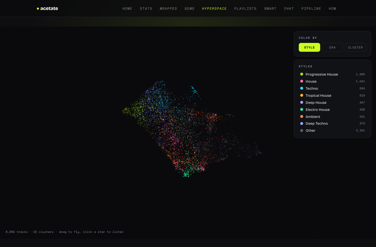
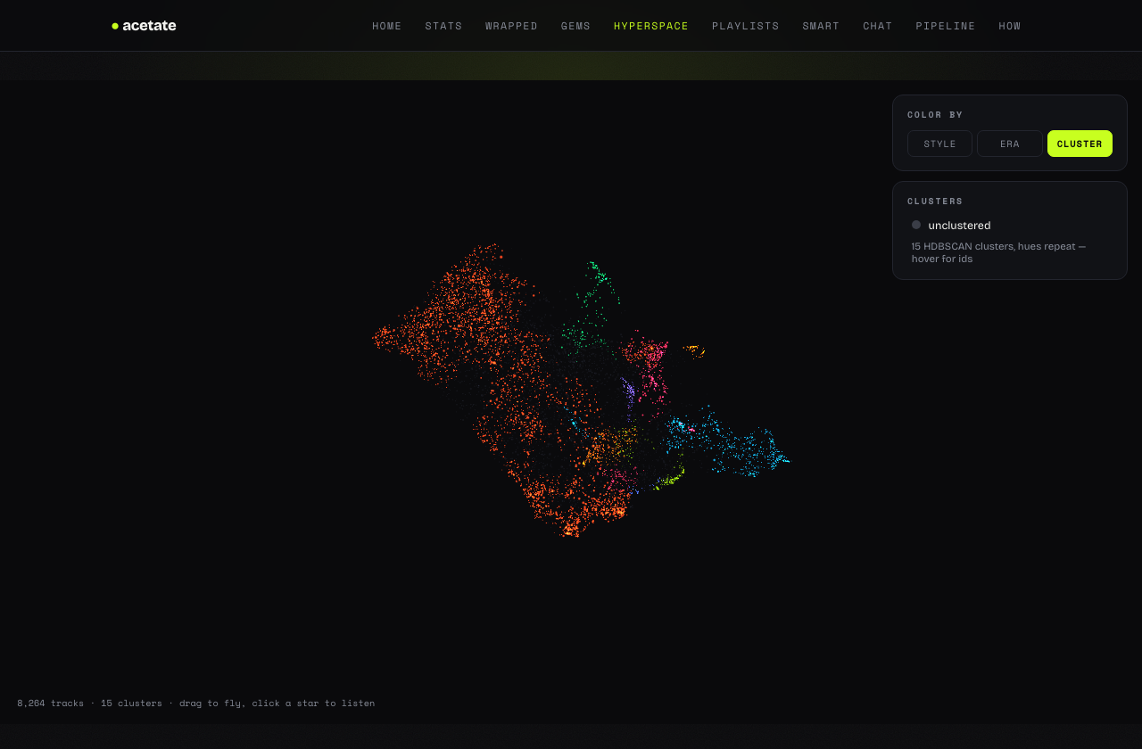
Then UMAP squashes 1280 dimensions to 3 while preserving neighborhoods, HDBSCAN finds the natural clumps, and three.js renders the result as a point cloud you can fly through: 24,163 stars, color by style, era, or cluster; size by play count; click a star and it plays. My taste turns out to have geography, a downtempo continent, a house peninsula, a trance archipelago drifting off on its own.
Under the hood: UMAP + HDBSCAN
The map is two more model choices, and both fields are crowded, so: the space, the pick, the mechanics.
Getting 1,280 dimensions down to three. The classic menu: PCA is linear, it finds the axes of maximum variance, which is perfect for compression and useless for maps, because neighborhoods aren't linear and the clusters smear into one another. t-SNE made the beautiful-scatterplot era: it preserves local neighborhoods well but famously mangles the global layout, distances between clusters mean nothing, and every run is a one-off: no reusable transform for new points, and it crawls at scale. UMAP keeps t-SNE's local fidelity, does meaningfully better on global arrangement, chews through thousands of 1280-d vectors in seconds, and, the deciding feature here, learns a reusable transform, so a newly embedded track can land in the existing map without recomputing the world. (PaCMAP and friends refine the trade-offs further; UMAP is the point on the curve with the ecosystem.)
How UMAP actually works, compressed but not lied about: it assumes the data sits on a lower-dimensional curved surface inside the 1280-d space, builds each point's k-nearest-neighbor graph, and converts distances into fuzzy edge weights, adaptively per point, so dense regions and sparse ones both stay connected. Then it scatters the points into 3D and runs a tug-of-war: attraction along real edges, repulsion against randomly sampled non-neighbors, word2vec's negative-sampling trick, applied to geometry, until the 3D graph agrees with the high-dimensional one. The standard caveat, worth saying out loud: after that much violence to the geometry, trust the neighborhoods, not the distances. Which is fine, the map is for flying; the actual similarity math runs brute-force in the full space (next section).
Finding the clumps. Same drill. k-means wants the number of clusters up front (I don't know how many scenes my taste has), insists they're round (taste isn't), and drafts every point into a cluster (a library has oddballs). DBSCAN fixed the shape and noise problems, a cluster is any dense region, whatever its shape, and loners stay unlabeled, but it runs at a single density threshold, and no one number works when the downtempo continent is packed and the outskirts are sparse. HDBSCAN is DBSCAN at every density at once: inflate distances in sparse neighborhoods (mutual reachability), build the minimum spanning tree, peel edges longest-first, which replays the clustering across the entire density range, and keep the clusters that persist longest across that sweep. "Choose k" becomes "keep what survives," the only real knob is a minimum cluster size, and points that belong nowhere are allowed to belong nowhere. That last property is load-bearing: the gray arm of the map is real, and pretending it's a genre would be a lie told in color.
Teaching it to read
A 400-style taxonomy, however deep, can't express "hypnotic dub techno, no vocals, long build." That sentence isn't a class, it's a description, and matching descriptions to sound needs a model that speaks both. Enter CLAP (Contrastive Language-Audio Pretraining), which is the CLIP trick ported to sound.
Under the hood: CLAP
Two encoders, one space. An audio encoder (HTSAT, a transformer that attends over spectrogram patches instead of convolving over them) maps a clip to a 512-d vector; a text encoder (RoBERTa) maps a caption to a 512-d vector. Training shows the pair hundreds of thousands of (audio, caption) examples and applies a contrastive loss: in every batch, pull each clip toward its own caption and push it away from everyone else's,
where τ is a temperature and sim is cosine. This training does not teach the model classes; it teaches it a shared geometry where sound and language about sound land near each other. That buys the magic property: any text, including text no one ever trained on, becomes a point in audio space, and retrieval is the same cosine-and-argsort we already run for sonic neighbors. Free-text search over a music library, zero classifiers involved.
And you can literally look at that shared geometry. Below: all 8,264 songs' CLAP audio vectors reduced to 2D, with eight sentences pushed through the text tower and projected into the very same map:
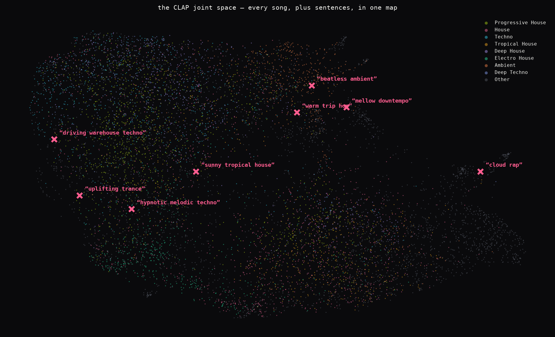
The trade. Where effnet's space is genre-shaped (that was its exam), CLAP's is
description-shaped: it's strongest on instrumentation, mood, production texture, the
things people write in captions, and weaker on micro-genre sociolects like "melodic techno,"
which appear in captions rarely. That's why it complements rather than replaces the other two
signals. And one scar from the DISCO autopsy, promoted to a rule: the checkpoint is pinned
(music_audioset_epoch_15_esc_90.14) and baked into the embeddings' model id ,
vectors from different CLAP checkpoints do not share a space, and an unpinned checkpoint is a
dataset nobody can ever join against.
The objective, caught in the act. Eight tracks, one per Discogs style; eight text descriptions, one aimed at each. If contrastive training did its job, the bright cells should walk the diagonal, pink outline marks where the "right" answer lives, lime marks what the model actually picked:
| PeriphescenceGlowworm | Gold - Thomas Jack Radio EditGabriel Rios | Electric EyesMetaform | Laminar FlowTommy Baynen | Silent ShoutThe Knife | Saving LightGareth Emery | Cut Your Teeth - Kygo RemixKyla La Grange | NevergreenEmancipator | |
|---|---|---|---|---|---|---|---|---|
| “beatless ambient soundscape with slowly evolving pads” | 0.11 | -0.02 | -0.02 | 0.08 | -0.05 | 0.04 | 0.01 | -0.02 |
| “deep house groove with a warm rolling bassline” | 0.22 | 0.30 | 0.20 | 0.25 | 0.17 | 0.31 | 0.39 | 0.07 |
| “mellow downtempo electronica with a dusty beat” | 0.33 | 0.24 | 0.35 | 0.23 | 0.17 | 0.20 | 0.25 | 0.20 |
| “progressive house with a long melodic build” | 0.17 | 0.28 | 0.14 | 0.32 | 0.18 | 0.33 | 0.34 | 0.07 |
| “dark pulsing electronic with eerie vocals” | 0.17 | 0.32 | 0.32 | 0.35 | 0.24 | 0.38 | 0.33 | 0.13 |
| “uplifting trance anthem with soaring supersaws” | 0.12 | 0.27 | 0.26 | 0.45 | 0.27 | 0.54 | 0.43 | 0.08 |
| “sunny tropical house with a bouncy summer feel” | 0.15 | 0.36 | 0.18 | 0.30 | 0.20 | 0.35 | 0.43 | 0.06 |
| “trip hop with boom-bap drums and moody atmosphere” | 0.27 | 0.33 | 0.37 | 0.18 | 0.18 | 0.16 | 0.16 | 0.30 |
Four of eight land exactly on the diagonal, and the misses are the real finding: ambient, downtempo, trance, and tropical house resolve correctly, while the deep house / progressive house / techno prompts scatter among each other's tracks, sibling styles inside one family. CLAP separates families crisply and blurs siblings; the supervised discogs space is sharpest exactly at sibling level, because telling siblings apart was its exam. Together they make a two-model system. (Negative result, dutifully logged: rewriting the prompts as rich captions instead of bare genre words did not improve the diagonal, 4/8 either way. The ceiling is the space, not the phrasing.)
Live demonstration, real numbers. Cosine similarity between five text prompts and five tracks from this year's rotation, computed with the actual model against the actual preview audio (shading is per-row relative; the outlined cell is each prompt's winner):
| Listen to the SilenceCorren Cavini | Senza FineEarthLife | endless nighteenspire | StardustOscuro | Closerstxrless | |
|---|---|---|---|---|---|
| “melodic techno with a hypnotic build” | 0.36 | 0.31 | 0.27 | 0.24 | 0.32 |
| “driving dark warehouse techno” | 0.26 | 0.27 | 0.21 | 0.23 | 0.26 |
| “warm mellow downtempo with a dusty beat” | 0.12 | 0.18 | 0.34 | 0.30 | 0.18 |
| “dreamy ambient textures, spacious reverb” | 0.16 | 0.12 | 0.13 | 0.13 | 0.15 |
| “moody lo-fi cloud rap with vocals” | 0.16 | 0.10 | 0.25 | 0.15 | 0.25 |
Four of five prompts pick the right track. The fifth, "dreamy ambient textures", comes back flat everywhere, and that's the honest reading: none of these five is actually beatless, and the model refuses to pretend otherwise. Grading note for the skeptical: prompt phrasing moves absolute scores, which is why the shading is per-row. repro: scripts/clap_worker.py matrix
Roads not taken (but properly scouted)
Half of building something like this is deciding what not to build. The graveyard, with justifications, because the reasoning is the reusable part:
The obvious move, search YouTube for "artist - title", download, embed. My instinct was that YouTube audio quality would be the problem. Wrong on both counts: quality is irrelevant (the model hears 16 kHz mono; see above), and the actual problems are matching, search happily hands you the live version, the sped-up edit, the re-upload, and pace: bot-throttling means seconds-per-track politeness, a multi-day trickle for 8k tracks. Deezer's ISRC lookup is an exact-match oracle by comparison, and an afternoon instead of a week. yt-dlp survives only as a last resort for the ~5% preview misses.
The community tooling that pulls full lossless tracks out of a paid streaming account , ISRC-exact, real quality. Set aside on every axis that matters here: for embeddings it buys literally nothing (16 kHz mono, again), the tooling is semi-maintained and squarely against the ToS with account-ban risk to match, and quality-for-humans is what the Spotify link is for. The itch it points at, a collection with no single point of failure, is real, but that's a storage problem, not an analysis one, and not this project's to solve.
The zero-infra option: POST each clip to a hosted discogs-effnet. But you still have to acquire the audio locally first, at which point the "zero infra" is a per-call bill for a model that runs at 0.8s/track on the laptop already sitting here. Local wins on cost, privacy, and not uploading 4GB of clips.
The textbook first move: export vectors.tsv + metadata.tsv, drop them into projector.tensorflow.org, get a free 3D UMAP in the browser. Genuinely the fastest dopamine route, and the right call for most projects. Skipped here only because the dashboard already existed with its own aesthetic and audio serving, going straight to a custom three.js page meant click-to-play and legend isolation on day one instead of porting them later.
The deployed box runs everything else on a scheduler, so why not this? Because the embed stack is a one-time backfill plus occasional top-ups, not a 24/7 job, and containerizing TensorFlow would triple the image for something the laptop does in an afternoon. The pipeline is plain CLI jobs, so if top-ups ever become annoying, moving them to the box is a compose-file change, not a rewrite.
Similarity, two ways
"Similar" means two different things, and a good recommender needs both. Sonic similarity, this sounds like that, falls out of the embeddings for free. Each track is a unit-normalized vector, and similarity is just the cosine:
At library scale there's no vector database, no index, no service: 8k×1280 floats is 40 MB, and one numpy matrix-vector product scans all of it in a millisecond. Brute force is the architecture. Collaborative similarity, people who play this also play that, is the thing no amount of audio analysis produces, because it encodes human context: scenes, eras, DJ sets, mood associations. That signal has to come from somewhere with listeners.
The plan was ListenBrainz, the open-source listening commons, with a Labs API serving
exactly the "similar recordings" dataset I wanted, keyed by MusicBrainz IDs. I built the whole
ISRC→MBID resolution ledger to join against it… and every single query returns an empty list.
The API returned [] for everything, including Radiohead's "Creep". The dataset
behind the endpoint is currently unpopulated. Experimental infrastructure is like that; the
MBIDs are banked for whenever it comes back.
Also scouted: DISCO-10M, an academic dataset that shipped precomputed CLAP embeddings for ten million tracks, "similarity search over music you've never touched" as a download. It turned out to be dead, and the forensics are a story in themselves. No DMCA exists, Hugging Face publishes every takedown notice it receives, and none names it. The org page survives, emptied by its own members. The tell is what the same ETH group released afterwards: datasets with a Spotify-shaped hole, no preview URLs, no embeddings computed from Spotify audio, and a new legal disclaimer. Verdict: a quiet author-side takedown, almost certainly Spotify-ToS exposure. No public mirror survives, yet at least five research groups verifiably trained on retained copies through 2025, the data isn't gone, it's just unspeakable. And even alive it carried a fatal flaw: the CLAP checkpoint behind its vectors was never documented, and embeddings from different checkpoints don't share a space, so you could never have reliably joined your vectors to theirs anyway. And track2vec on the Million Playlist Dataset , word2vec over a million playlists, tracks as words, is real and clever, but the dataset froze in November 2017, which for electronic music is a different geological era.
So collaborative duty falls to Last.fm's getSimilar, alive, good, and pleasantly humble, and the roadmap engine stacks the spaces instead of picking one:
Candidates the library has never seen get embedded on demand, name → Deezer preview → 0.8 seconds of inference, and land in the same space as everything else, compatible by construction. A recommendation engine whose only user I have to please is me.
The agent
The chat page is an LLM agent with exactly three tools: a read-only SQL query layer (read-only connection, single-SELECT guard, row caps, timeouts), a similar-tracks tool that answers from both similarity spaces at once (SQL can't do cosine math on blobs, so this one earned a real tool), and a propose-playlist tool whose output is a card I approve or ignore, the model can suggest, never act. And a hard rule sits under all of it: every playlist write in the codebase goes through a gate that verifies acetate created that playlist. There is no code path that deletes or edits a playlist I made by hand. The blast radius of any bug, agent tantrum included, is "a robot playlist got weird".
The boring parts, done stubbornly
FastAPI + HTMX + inline Jinja templates, the whole UI ships in one Python file, no bundler.
Secrets resolve from 1Password references in dev and plain env on the box. Deploys are
just deploy.
One war story earns its paragraph. SQLite in WAL mode allows exactly one writer at a
time, and a write transaction holds that lock from its first statement until commit. The
embed worker batched its commits every 50 tracks, 40 seconds of inference per batch, which
meant 40-second lock holds while the preview fetcher and the MusicBrainz resolver queued up
behind it until one of them blew past its 30-second busy timeout and died with
database is locked. The fix is the general rule: commit per unit of work.
A commit costs a millisecond; holding the only write lock across a neural-net call costs you
your other two pipelines. With short transactions, three concurrent backfills plus the poller
plus the dashboard coexist on one file without a murmur. Similar story in the fetcher: going
from serial requests to four worker threads behind one shared rate-limiter turned a six-hour
download into 45 minutes, with the DB writes kept on the main thread so the lock never crosses
a thread boundary.
What's next
Genre playlists that curate themselves (the discogs styles finally give the classifier real input), the retrieve→rerank→sequence playlist engine, natural-language search over the audio space ("hypnotic dub techno, no vocals" → CLAP embedding → tracklist), lasso-select in Hyperspace → instant playlist, and a full lossless mirror of the collection on the NAS, because the whole premise of this project is that my listening history shouldn't have a single point of failure I don't own.
Field notes, the worklog
This isn't a finished-project writeup; it's the start of one. Everything tried, wins, dead ends, and faceplants alike, gets logged below as it happens. Newest first.
First sip from YouTube Music radio. The unofficial YouTube Music client surface is exactly as strange and useful as advertised: give it one seed track, ask for radio, and it returns a generated queue. Wired the first conservative harvester today. It resolves known songs through the local LAION-DISCO catalog before falling back to YT Music search, asks for radio queues, and stores every returned track as another provenance edge in the candidate ledger. First polite runs: 33 seeds → 1,139 stored radio edges, with 30 of 50 high-play seeds resolved straight from the local catalog. Title cleanup is deliberately lookup-only, exact titles first, version suffixes only as fallback keys, originals preserved. This is the kind of surface that may vanish without warning, so the rule is simple: cache raw responses, use it politely, and never make it the only leg of the table.
The recommendation frontier gets a ledger. The next problem is finding music outside the library without trying to download the world. First piece landed: a provenance-first candidate ledger. Last.fm's out-of-library co-listening graph now becomes 142,796 metadata candidates backed by 355,799 reasons: which known track led there, what source said so, and how strong the edge was. Independent weak signals can now accumulate before acetate spends money or compute on previews and embeddings.
The spectrogram confesses. The full-track figure's section lines were eyeballed, and wrong, what was labeled the breakdown was a 17-second break at 2:13; the real breakdown is the 29-second kick-out at 2:54, and the groove enters at 0:30, not 0:50. Fixed by computing the sub-150 Hz kick-band energy envelope and reading the on/off transitions instead of squinting. The annotated arc now matches the audio: groove 0:30 → break 2:13 → breakdown 2:54 → drop 3:25 → stripped DJ outro 4:26. Lab-notebook rule, reaffirmed: annotations are claims, and claims get measured.
The whole library, mapped. Backfill complete. Every track played at least once in fourteen years, plus everything ever liked: 24,163 recordings fetched (79.6% preview coverage, 6,184 the catalogs simply don't carry), embedded in all three models with zero errors, projected into both spaces (47 and 41 clusters). The map tripled in a day. Alongside it: 468k co-listening edges and 17.7k MusicBrainz IDs. Five external sources, three neural nets, two embedding spaces, one SQLite file.
The features Spotify took away came back. Chased a half-remembered rumor of a 'Spotify data leak.' Verdict: no breach ever, but Anna's Archive scraped ~300TB of the catalog in Dec 2025, and a 56M-track extract of the classic audio features (energy, valence, tempo, danceability…) now sits openly on Hugging Face, keyed by Spotify track id. The Echo Nest built those numbers, Spotify buried them in Nov 2024, and the commons dug them back up, for any library that still remembers its track ids, the features the API refuses to serve are one exact-ID join away. Filed next to the DISCO autopsy: the metadata economy giveth, and the metadata economy is leaky.
The product catches up to the data. Hyperspace v2 adds track search with a fly-to camera, a metadata sidebar, nearest-neighbors you can hop along like stepping stones, CLAP text queries, liked/min-plays filters, and a space toggle between effnet's genre-shaped projection and CLAP's description-shaped one. CLAP embeds each track directly from audio and needs no labels; the colors are just paint on top.
CLAP gets the full anatomy and a two-model thesis. Two new figures: the joint-space map (all 8,264 songs in CLAP space with eight sentences projected into the same plane, “cloud rap” lands on the hip-hop island, the ambient prompts on the ambient coast) and the 8×8 diagonal experiment: one track per style vs one description per track. 4/8 exact, and every miss stays within the right family. Finding: CLAP separates families, discogs-effnet separates siblings, a two-model system, not redundancy. Bonus negative result: caption-rich prompts didn't beat bare genre words.
DISCO hunt: a fragment recovered. Round-2 forensics found live survivors: Andrew Gao's DISCO-200K-Tensors (410 MB of embeddings + song index derived from the 200K-high-quality subset), still on Hugging Face, now preserved locally, SHA-verified, and a Chinese mirror holding the complete 147-shard file manifest of the full 10M behind a free login (bytes unverified). The dataset is Schrödinger-alive: everyone has it, nobody hosts it.
The specimen gets a full anatomy. Added a 4-second zoom of the specimen (count the kick columns; note how much more of the log-mel canvas carries texture) and a full-track spectrogram with the arc annotated, intro, breakdown wedge, the drop, structure that's invisible to the 30s preview, the ~3s model patches, and the mean-pooling alike. Fine for vibe; a per-section index is the natural sequel. Bonus honesty: yt-dlp served the 5:30 extended mix for the 3:49 edit, the graveyard section's matching hazard, live.
The explainers get real data. Every model section now uses my library: a linear-vs-log-mel spectrogram pair of Corren Cavini's “Listen to the Silence” (16 kHz mono, the network's input), its discogs400 activations, and a live 5×5 CLAP prompt×track cosine matrix. Four of five prompts pick the intended track; the fifth honestly shrugs. Repro scripts committed.
DISCO-10M: cause of death established. Forensics found no DMCA. Hugging Face publishes every takedown notice it receives and none names DISCOX; the org page survives, emptied by its own members. Everything the ETH group shipped afterwards has a Spotify-shaped hole: no preview URLs, no Spotify-derived embeddings, and new legal disclaimers. The evidence points to an author-side removal over Spotify ToS exposure. No public mirror survives, although at least five labs verifiably trained on retained copies through 2025. The data isn't gone; it's unspeakable.
CLAP hears “melodic techno”: early verdict. With the CLAP backfill only a third done, asked it for “melodic techno with a long hypnotic build”: Anyma, Joris Voorn, The Element MT, James Trystan, Afterlife-core, all liked, retrieved from text alone, even where the Discogs taxonomy calls them Progressive House. The query the entire genre saga failed at, answered by a model that has never seen a genre label. One impostor (Alan Walker) in eight. Checkpoint pinned to music_audioset_epoch_15, the DISCO lesson, institutionalized.
The co-listening graph gets persisted. Last.fm getSimilar was being fetched live and thrown away. Now it's cached: ~50 edges per track with match scores, plus global listeners/playcount, the obscurity signal no tag carries. First dozen seeds: 599 edges, 28% pointing back into the library. This is the collaborative substrate for genre label-propagation and the playlist engine's retrieve stage. Also pinned the genre-classifier plan: three signals, discogs400 styles, raw embeddings with my own playlists as labeled regions, Last.fm tags, judged against my authored playlists as ground truth.
The blog becomes a lab notebook. Reframed this page as a running log. Every experiment from here lands in this section, including the ones that die.
The agent learns “more like this”. New similar_tracks chat tool answering from both spaces in one call, and the SQL tool now knows the styles table. First test: Bakermat → ZHU, Jamie xx (sonic) / Klangkarussell, Kygo (collaborative). The playlist-maker has ears now.
DISCO-10M autopsy. Hoped to buy 10M precomputed CLAP vectors and search music I've never owned. The dataset's been pulled from Hugging Face, no mirror, and the model checkpoint was never documented, its vectors were never joinable anyway. Verdict: embed candidates on demand into our own space; names are cheap, vectors we make ourselves.
Full map, and a locked database. All 8,264 fetched clips embedded overnight, zero errors, 15 clusters. Along the way: three backfills on one SQLite file taught me WAL's single-writer rule the hard way (database is locked), fixed by committing per unit of work instead of batching commits across 40s of inference.
ListenBrainz returns []. Built the full ISRC→MBID ledger to join their similar-recordings dataset… which currently returns an empty list for every recording on Earth, Radiohead included. MBIDs banked for when it repopulates; collaborative duty reassigned to Last.fm getSimilar.
First light. 845 stars, first flight through the library. Also the day's two best bugs: a shader that rendered pure black because three.js doesn't declare custom uniforms for you, and a cloud 10× too small from scaling coordinates before centering them.
The Deezer discovery. ISRC → exact 30s preview from a public API, no account: 5/5 on the first probe. Killed the whole yt-dlp download plan in one afternoon. Threading the fetcher behind one rate-limiter took the run from ~6h to ~45min.
Decisions pinned. Universe = liked ∪ ≥5 plays (8,689 recordings). Previews only, the 16 kHz-mono resampler makes 128 kbps lossless to the model. Local Mac compute in isolated script envs. Straight to a custom map page, no Embedding Projector detour.
Coda
Fourteen years of listening, one neural network's opinion of it, three dimensions. On the box it hangs in space as a live map, 24,163 stars you can fly through, click, and play. A curated cut of it is live on this site: coordinates and names only, no listening data attached.
Built with: Python 3.12 + uv · SQLite · FastAPI + HTMX · spotipy · Last.fm API ·
MusicBrainz · Deezer previews · essentia-tensorflow (discogs-effnet, CC BY-NC-ND, personal use) ·
umap-learn · scikit-learn HDBSCAN · three.js · Docker. No cloud, no telemetry, no build step.
This page is a static snapshot of the living lab notebook that runs on the box itself ,
numbers baked from the real database on 2026-07-05.